Actuarial calculations are often inputs in the regulatory, accounting, and financial budgeting needs of clients of all sizes. For companies that sponsor single-employer defined benefit pension plans, actuarial calculations are required in determining the minimum required contribution under the Employee Retirement and Income Security Act of 1974 (ERISA) and the net periodic pension cost under Financial Accounting Standards Board Accounting Standards Codification (ASC) subtopic 715 for companies who report under GAAP.
The output of these types of actuarial calculations is a fixed “answer.” The answer flows mathematically from the calculations, based on the census data provided by the plan sponsor, the computer programming of promised benefits, and the assumptions that are selected for the measurement. The models that produce these fixed “answers” are known as deterministic models.
Limitations to deterministic models
It is important to understand that the required calculations under ERISA and GAAP only reveal a partial picture of reality. They do not account for deviations and do not provide clarity on risk. In addition, these models and results do not adequately communicate to the plan sponsor the sensitivity of results to deviations in inputs—for example, changes in census data, benefits offered, or volatility in capital markets. Instead, actuaries tend to think in terms of reasonable ranges rather than fixed answers.
The sensitivity of changes in census data and benefit offerings can be analyzed using experience studies and plan design projects, respectively. The sensitivity of results to volatility in capital markets can be communicated in two ways:
- Deterministic modeling, via stress testing or sensitivity analysis, in which the actuary produces results along several selected deterministic tracks to show how the outputs change given changes in asset returns, interest rates, and inflation, providing “pessimistic” and “optimistic” results rather than a single answer
- Stochastic modeling, in which the actuary produces a range of results, rather than a single answer, that correspond to hundreds or thousands of different simulated economic scenarios
Advantages to stochastic modeling
While both techniques allow a plan sponsor to get a sense of the risk—that is, the volatility of outputs—that is otherwise opaque in the traditional single deterministic model, stochastic modeling provides some advantage in that the individual economic scenarios are not manually selected. Rather, a wide range of possible economic scenarios, based on a set of capital market assumptions, are simultaneously analyzed to provide the range of possible outcomes and the likelihood of occurrence.
Stochastic models are particularly useful in forecasting, in which the actuary produces estimates of results in future years, not just a current year valuation. The output of the model will show not only the underlying riskiness of an output variable—for example, funded status or contribution requirements—but also how the risks may change over time.
Examples of deterministic forecasts
Consider the following output of a deterministic forecast model showing a pension plan’s projected funded status over the next five years. In developing this model, the actuary has assumed that interest rates will remain flat over the five-year period and that the plan’s assets will experience an annual return equal to the plan sponsor’s expected return on asset assumption for financial reporting under ASC 715.
Figure 1: Five-year projected funded status, assuming unchanged interest rates
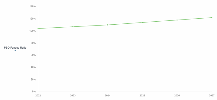
The results show one possible scenario. An actuary could create a stress test by developing an alternative deterministic forecast with different assumptions. For example, the actuary could produce a forecast that assumes interest rates will increase 50 basis points (bps) for each of the next two years before leveling off, as illustrated in Figure 2.
Figure 2: Alternative forecast assuming interest rates rise 100 bps over a two-year period
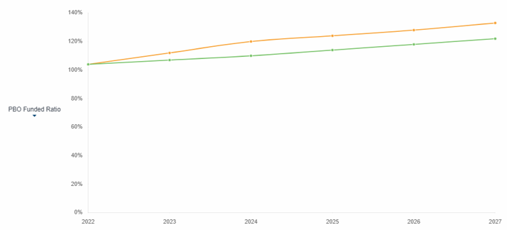
Viewing these two forecasts provides the plan sponsor an idea of how sensitive the plan’s funded status is to changes in interest rates. However, it is limited in that the sponsor is only seeing the impact of two selected economic scenarios.
Examples of stochastic forecasts
In a stochastic forecast, the actuary uses a set of capital market assumptions (CMAs), typically developed by an investment consultant, to generate a large set of economic simulations. CMAs specify the expected return and volatility of a variety of asset classes. In addition, the CMAs will indicate the correlation among the asset classes. From these CMAs, a diverse set of future economic environments can be forecast, rather than be limited to one or two selected scenarios.
Instead of a single projected funded status for each future year, the stochastic forecast provides a range of possible funded statuses for each future year, along with percentile data to show the likelihood of these results.
Figure 3: Stochastic forecast showing a range of possible outcomes
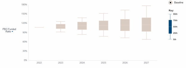
The results of a stochastic forecast can be illustrated in the form of a floating bar chart, sometimes known as a “box and whisker” chart, as in Figure 3. For each year, the floating bar chart represents the range of possible outcomes between the 5th percentile (indicating that only 5% of scenarios were lower) and the 95th percentile (indicating that 95% of scenarios were lower, meaning that only 5% of scenarios were higher).
The central bar, or the “box,” represents the middle 50% of all forecasted scenarios—that is, from the 25th to the 75th percentile. This means that half of all forecasted scenarios fell within this range. We can see in Figure 4 below that the plan’s funded status for 2023 is between 103% and 117% in half of the simulations. Another way to interpret this chart is to note that 25% of the simulations resulted in a funded status above 117% and the other 25% of the simulations resulted in a funded status below 103%.
Figure 4: Box-and-whisker chart illustrating financial risks of adverse economic environments
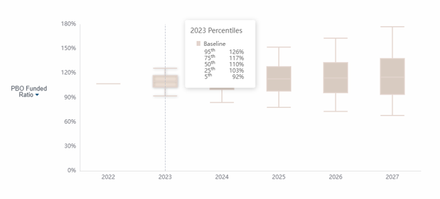
The tails, or “whiskers,” that stretch above and below the “box” represent the 20% of scenarios that were above and below the middle 50 percentile (i.e., 75th to 95th and 5th to 25th). In this chart, the 5% worst-case scenario was a funded status of 92%, while the 95% best-case scenario was a funded status of 126%. The whiskers allow the plan sponsor to understand the financial risks of adverse economic environments.
A complement to the floating bar chart is a target line chart. This graphic allows a plan sponsor to determine the percentage of scenarios that fell above a certain target percentage. In Figure 5 below, the target line has been placed at 110% of the projected benefit obligation (PBO) funded status, which sometimes is viewed as a proxy for a plan termination liability.
Figure 5: Target line chart illustrating the percentage of scenarios above a threshold
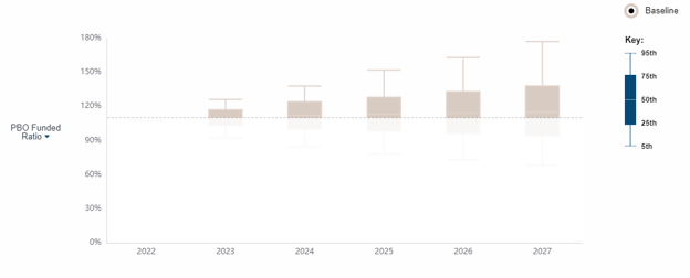
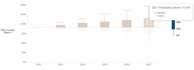
The plan sponsor can see in Figure 6 below that there is nearly a 56% probability that the plan will be more than 110% funded on a PBO basis by 2027.
Figure 6: Stochastic forecast with target line can help a plan sponsor with strategic planning
Closing
The concepts underlying stochastic models can be intimidating for first time users. Stochastic forecast results may, at first, appear to be quite complicated. But after the plan sponsor is oriented to the meaning of the output, the results of a stochastic forecast can lead to a significant increase in understanding of the risk and volatility facing a plan.